General Demo
This notebook serves as a demonstration of what the toolbox can do. This project is a work in progress, so there will be updates to the code and subsequently the applications. Below are some highlights of what is currently possible.
Datasets
The starting point of the project is the ability to easily load chemical datasets into a format that is usable from a Machine Learning perspective. All the relevant datasets make use of SMILES (Simplified molecular-input line-entry system) to store information on molecules. The in-built DataSet objects then take the SMILES representation of molecules together with a target array and any other additional information, and load then into graphs.
Below is an example of an implemented dataset that can, similarly to the torch datasets, download and load a dataset from the internet.
Jean-Claude Bradley Open Melting Point Dataset [1]
[2]:
from grape_chem.datasets import BradleyDoublePlus
print(f'length of dataset at the start: {3024}\n-------------')
data = BradleyDoublePlus(log=True, only_organic=True)
print(f'-------------\nlength of dataset at the end: {len(data)}')
length of dataset at the start: 3024
-------------
SMILES [O-][N+]#N in index 1 does not contain at least one carbon and will be ignored.
SMILES FS(F)(=O)=O in index 2 does not contain at least one carbon and will be ignored.
SMILES BrBr in index 4 does not contain at least one carbon and will be ignored.
SMILES II in index 8 does not contain at least one carbon and will be ignored.
SMILES ClS(Cl)(=O)=O in index 79 does not contain at least one carbon and will be ignored.
SMILES B(OCC)(OCC)OCC in index 144 contains the atom B that is not permitted and will be ignored.
SMILES c1cccn1 in index 308 is not valid.
SMILES N#Cc3cncc3c1cccc2OC(F)(F)Oc12 in index 370 is not valid.
SMILES CC[Si](CC)(CC)CC in index 519 contains the atom Si that is not permitted and will be ignored.
SMILES CC[Si](CC)(Cl)Cl in index 541 contains the atom Si that is not permitted and will be ignored.
SMILES [SiH](Cl)(Cl)Cl in index 565 contains the atom Si that is not permitted and will be ignored.
SMILES [SiH](Cl)(Cl)Cl in index 565 does not contain at least one carbon and will be ignored.
SMILES c1ccc(cc1)[Si](c2ccccc2)(c3ccccc3)c4ccccc4 in index 592 contains the atom Si that is not permitted and will be ignored.
SMILES c1ccc(cc1)[Si]2(O[Si](O[Si](O[Si](O2)(c3ccccc3)c4ccccc4)(c5ccccc5)c6ccccc6)(c7ccccc7)c8ccccc8)c9ccccc9 in index 605 contains the atom Si that is not permitted and will be ignored.
SMILES c1ccc(cc1)[Si]2(O[Si](O[Si](O[Si](O2)(c3ccccc3)c4ccccc4)(c5ccccc5)c6ccccc6)(c7ccccc7)c8ccccc8)c9ccccc9 in index 605 contains the atom Si that is not permitted and will be ignored.
SMILES c1ccc(cc1)[Si]2(O[Si](O[Si](O[Si](O2)(c3ccccc3)c4ccccc4)(c5ccccc5)c6ccccc6)(c7ccccc7)c8ccccc8)c9ccccc9 in index 605 contains the atom Si that is not permitted and will be ignored.
SMILES c1ccc(cc1)[Si]2(O[Si](O[Si](O[Si](O2)(c3ccccc3)c4ccccc4)(c5ccccc5)c6ccccc6)(c7ccccc7)c8ccccc8)c9ccccc9 in index 605 contains the atom Si that is not permitted and will be ignored.
SMILES C[Si]1(O[Si](O[Si](O[Si](O1)(C)C=C)(C)C=C)(C)C=C)C=C in index 626 contains the atom Si that is not permitted and will be ignored.
SMILES C[Si]1(O[Si](O[Si](O[Si](O1)(C)C=C)(C)C=C)(C)C=C)C=C in index 626 contains the atom Si that is not permitted and will be ignored.
SMILES C[Si]1(O[Si](O[Si](O[Si](O1)(C)C=C)(C)C=C)(C)C=C)C=C in index 626 contains the atom Si that is not permitted and will be ignored.
SMILES C[Si]1(O[Si](O[Si](O[Si](O1)(C)C=C)(C)C=C)(C)C=C)C=C in index 626 contains the atom Si that is not permitted and will be ignored.
SMILES COc1cc(cc(OC)c1OC)/C=C/C(=O)O[C@@H]3C[C@@H]4CN5CCc2c6ccc(OC)cc6nc2[C@H]5C[C@@H]4[C@@H]([C@H]3OC)C(=O)OC in index 662 is not valid.
SMILES c1cncn1 in index 697 is not valid.
SMILES c1cccc2nccc12 in index 698 is not valid.
SMILES Cc1cc2nnnc2cc1 in index 728 is not valid.
SMILES C[Si]1(C)O[Si](C)(C)O[Si](C)(C)O[Si](C)(C)O1 in index 734 contains the atom Si that is not permitted and will be ignored.
SMILES C[Si]1(C)O[Si](C)(C)O[Si](C)(C)O[Si](C)(C)O1 in index 734 contains the atom Si that is not permitted and will be ignored.
SMILES C[Si]1(C)O[Si](C)(C)O[Si](C)(C)O[Si](C)(C)O1 in index 734 contains the atom Si that is not permitted and will be ignored.
SMILES C[Si]1(C)O[Si](C)(C)O[Si](C)(C)O[Si](C)(C)O1 in index 734 contains the atom Si that is not permitted and will be ignored.
SMILES C in index 819 consists of less than 2 heavy atoms and will be ignored.
SMILES c1ccc(cc1)[SiH](c2ccccc2)c3ccccc3 in index 842 contains the atom Si that is not permitted and will be ignored.
SMILES Br in index 903 consists of less than 2 heavy atoms and will be ignored.
SMILES O=S=O in index 905 does not contain at least one carbon and will be ignored.
SMILES O=C(OC)[C@@]2(C[C@H]4C[C@@](O)(CC)C[N@@](CCc1c3ccccc3nc12)C4)c5cc9c(cc5OC)N(C=O)[C@@H]6[C@]98CCN7CC=C[C@@](CC)([C@@H](OC(C)=O)[C@]6(O)C(=O)OC)[C@H]78 in index 933 is not valid.
SMILES C[Si](C)(C)C in index 935 contains the atom Si that is not permitted and will be ignored.
SMILES [O-][N+](=O)c1ccc2ncnc2c1 in index 1305 is not valid.
SMILES [O-][N+](=O)c1cnc(C)n1 in index 1364 is not valid.
SMILES ClS(Cl)=O in index 1384 does not contain at least one carbon and will be ignored.
SMILES C[Si]1(N[Si](N[Si](N[Si](N1)(C)C)(C)C)(C)C)C in index 1732 contains the atom Si that is not permitted and will be ignored.
SMILES C[Si]1(N[Si](N[Si](N[Si](N1)(C)C)(C)C)(C)C)C in index 1732 contains the atom Si that is not permitted and will be ignored.
SMILES C[Si]1(N[Si](N[Si](N[Si](N1)(C)C)(C)C)(C)C)C in index 1732 contains the atom Si that is not permitted and will be ignored.
SMILES C[Si]1(N[Si](N[Si](N[Si](N1)(C)C)(C)C)(C)C)C in index 1732 contains the atom Si that is not permitted and will be ignored.
SMILES C[Si](C)(C)[Si](C)(C)C in index 1750 contains the atom Si that is not permitted and will be ignored.
SMILES C[Si](C)(C)[Si](C)(C)C in index 1750 contains the atom Si that is not permitted and will be ignored.
SMILES c1cccc2ncnc12 in index 1820 is not valid.
SMILES B(c1ccccc1)(O)O in index 1983 contains the atom B that is not permitted and will be ignored.
SMILES CC[SiH2]CC in index 2256 contains the atom Si that is not permitted and will be ignored.
SMILES c1ccc(cc1)[Si](c2ccccc2)(c3ccccc3)Cl in index 2268 contains the atom Si that is not permitted and will be ignored.
SMILES CC(=O)O[Si](C)(OC(=O)C)OC(=O)C in index 2316 contains the atom Si that is not permitted and will be ignored.
SMILES C[Si](c1ccccc1)(c2ccccc2)c3ccccc3 in index 2325 contains the atom Si that is not permitted and will be ignored.
SMILES Cc2cnc1ccccc12 in index 2335 is not valid.
SMILES c1ccc(cc1)[Si](c2ccccc2)(c3ccccc3)O in index 2390 contains the atom Si that is not permitted and will be ignored.
SMILES c1cccc2nnnc12 in index 2516 is not valid.
SMILES B(c1ccccc1C)(O)O in index 2674 contains the atom B that is not permitted and will be ignored.
SMILES CCO[Si](OCC)(OCC)OCC in index 2681 contains the atom Si that is not permitted and will be ignored.
SMILES n2cnc(NCc1ccccc1)c3ncnc23 in index 2686 is not valid.
SMILES B(c1ccccc1)(c2ccccc2)OCCN in index 2741 contains the atom B that is not permitted and will be ignored.
SMILES C[Si](C)(C)C#C[Si](C)(C)C in index 2775 contains the atom Si that is not permitted and will be ignored.
SMILES C[Si](C)(C)C#C[Si](C)(C)C in index 2775 contains the atom Si that is not permitted and will be ignored.
SMILES n1c3ccccc3nc1c2cscn2 in index 2916 is not valid.
SMILES COB(OC)OC in index 2935 contains the atom B that is not permitted and will be ignored.
SMILES N[C@@H](Cc1cncn1)C(=O)O in index 2944 is not valid.
SMILES C[Si]1(C)O[Si](C)(C)O[Si](C)(C)O1 in index 3008 contains the atom Si that is not permitted and will be ignored.
SMILES C[Si]1(C)O[Si](C)(C)O[Si](C)(C)O1 in index 3008 contains the atom Si that is not permitted and will be ignored.
SMILES C[Si]1(C)O[Si](C)(C)O[Si](C)(C)O1 in index 3008 contains the atom Si that is not permitted and will be ignored.
SMILES Sc1nc2ccccc2n1 in index 3018 is not valid.
-------------
length of dataset at the end: 2989
As seen above, the data loader filters the SMILES based a few different criteria. One of them is a check if rdkit recognizes the SMILES representation as valid, another one is whether the SMILES atoms are all part of the allowed atom symbols. After filtering, we can access the information using the regular class notations.
Example outputs
We can access the SMILES from the melting point dataset as such:
[3]:
# SMILES
data.smiles[0:5]
[3]:
array(['CC1CCC1', 'CC(C)N(CCC(C(N)=O)(c1ccccc1)c1ccccn1)C(C)C',
       'CCn1cc(C(=O)O)c(=O)c2cc(F)c(N3CCNC(C)C3)c(F)c21', 'CN(C)C',
       'ClC(Cl)(Cl)Cl'], dtype=object)
And their corresponding graphs are stored at the same indices.
[4]:
# Their corresponding graphs, saved using the torch geometric Data objects.
data[0:5]
[4]:
[Data(x=[5, 44], edge_index=[2, 10], edge_attr=[10, 12], y=[1]),
 Data(x=[25, 44], edge_index=[2, 52], edge_attr=[52, 12], y=[1]),
 Data(x=[25, 44], edge_index=[2, 54], edge_attr=[54, 12], y=[1]),
 Data(x=[4, 44], edge_index=[2, 6], edge_attr=[6, 12], y=[1]),
 Data(x=[5, 44], edge_index=[2, 8], edge_attr=[8, 12], y=[1])]
We can draw any of the loaded SMILES using rdkit directly:
[5]:
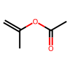
print('SMILES:', data.smiles[10])
print('Target: ', data.target[10], ' [Celsius]')
print('Graph Target: ', data.graphs[10].y, ' [Celsius]')
data.draw_smile(10)
SMILES: C=C(C)OC(C)=O
Target:  -93.0  [Celsius]
Graph Target:  tensor([-93.])  [Celsius]
[5]:
[6]:
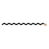
print('SMILES:', data.smiles[100])
print('Target: ', data.target[100], ' [Celsius]')
print('Graph Target: ', data.graphs[100].y, ' [Celsius]')
data.draw_smile(100)
SMILES: CCCCCCCCCCCCCCCCCCBr
Target:  28.0  [Celsius]
Graph Target:  tensor([28.])  [Celsius]
[6]:
[7]:
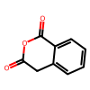
print('SMILES:', data.smiles[1000])
print('Target: ', data.target[1000], ' [Celsius]')
print('Graph Target: ', data.graphs[1000].y, ' [Celsius]')
data.draw_smile(1000)
SMILES: O=C1Cc2ccccc2C(=O)O1
Target:  142.0  [Celsius]
Graph Target:  tensor([142.])  [Celsius]
[7]:
We can also save and load the dataset as such:
[8]:
# We can also save and load the dataset as such:
# Datasets are saved using pickle, which allows for fast saving and loading. Saving a dataset and then loading instead of loading from, for example, an excel file is about 10 to 20 times faster.

from grape_chem.utils import DataSet

data.save_dataset('BradleyDoublePlus')
loaded_dataset = DataSet(file_path='./data/processed/BradleyDoublePlus.pickle')
loaded_dataset.smiles[0:5]
File saved at: ./data/processed/BradleyDoublePlus.pickle
Loaded dataset.
[8]:
array(['CC1CCC1', 'CC(C)N(CCC(C(N)=O)(c1ccccc1)c1ccccn1)C(C)C',
       'CCn1cc(C(=O)O)c(=O)c2cc(F)c(N3CCNC(C)C3)c(F)c21', 'CN(C)C',
       'ClC(Cl)(Cl)Cl'], dtype=object)
Datasets are saved using pickle, which allows for fast saving and loading. Saving a dataset and then loading from the pickle directly instead of regenerating it from the orignal data is about 10 to 20 times faster.
Analysis
There are several options to analyze a loaded dataset. Below are some of these options.
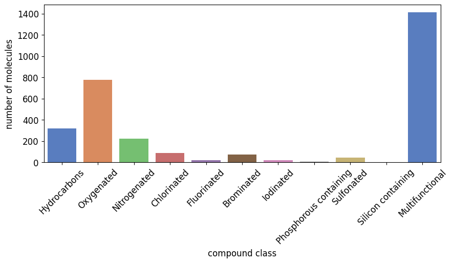
Naive clustering
This chart is generated using a simple clustering algorithm that checks the letter in the SMILES and puts them into the below seen molecule classes. For example, if a SMILES only contains an ‘O’ and no other class letter, then it is part of ‘Oxygenated’. If it contains ‘O’ and ‘Cl’, then it is part of ‘Multifunctional’.
[9]:
from grape_chem.plots import compound_nums_chart

compound_nums_chart(data.smiles, fig_size=(10,4))
[9]:
<Axes: xlabel='compound class', ylabel='number of molecules'>
Classyfire
An almost always more useful clustering is using the Classyfire [2] classification done by Feunang et al.. In code terms, we pull the online documentation of the molecules in question with their Classyfire information, read it and cluster them based on that. This approach is far superior over the simple one above, but can take very long to do (it takes about 2 min to retrieve the information for 100 molecules).
[10]:
subset_smiles = data.smiles[100:200]

from grape_chem.analysis import classyfire, classyfire_result_analysis
ids, data_ids = classyfire(subset_smiles, log=False)
smile_classes, class_num_dictionary = classyfire_result_analysis(idx=ids)
print(class_num_dictionary)
Found log file in working directory.
All passed smiles are already in the passed log_file.
Key error occurred using superclass for file 683.json.
Key error occurred using superclass for file 695.json.
Key error occurred using superclass for file 656.json.
Key error occurred using superclass for file 640.json.
Key error occurred using superclass for file 660.json.
Key error occurred using superclass for file 621.json.
Key error occurred using superclass for file 699.json.
Key error occurred using superclass for file 676.json.
{'Benzenoids': 37, 'Phenylpropanoids and polyketides': 1, 'Organic nitrogen compounds': 3, 'Organophosphorus compounds': 1, 'Organoheterocyclic compounds': 11, 'Organic oxygen compounds': 5, 'Organohalogen compounds': 13, 'Hydrocarbons': 9, 'Organic acids and derivatives': 7, 'Acetylides': 1, 'Lipids and lipid-like molecules': 2, 'Alkaloids and derivatives': 1, 'Organosulfur compounds': 1}
[11]:
from grape_chem.plots import num_chart
num_chart(class_num_dictionary, fig_size=(10,4))
[11]:
(<Figure size 1000x400 with 1 Axes>,
 <Axes: xlabel='compound class', ylabel='number of molecules'>)
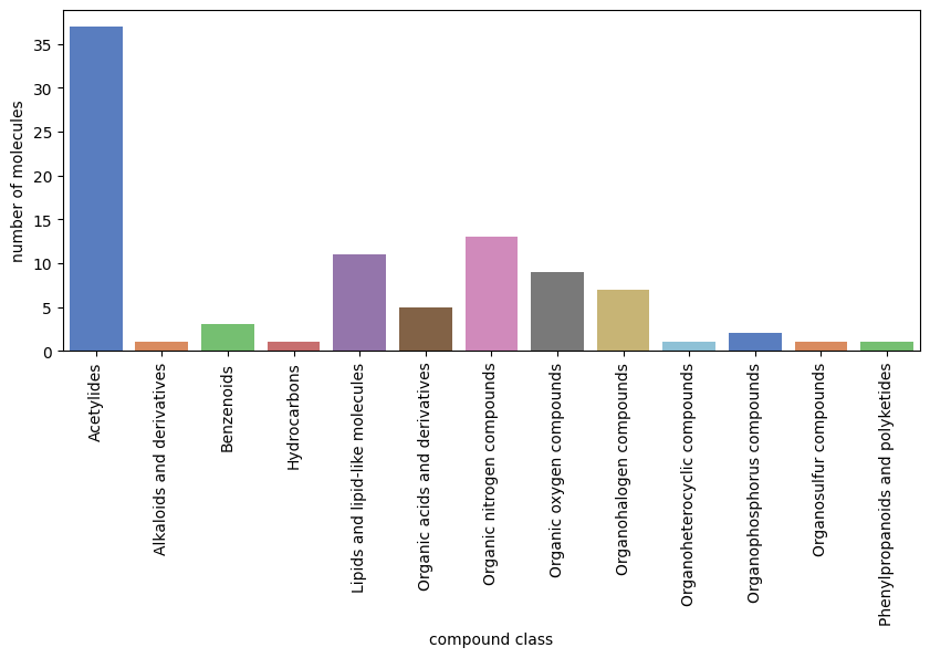
The classyfire code is split in two: (1) classyfire sends the relevant information to the classyfire website (http://classyfire.wishartlab.com/) and retrieves the class information as a json file. Furthermore, a csv file called recorded_SMILES is generated that stores the json file indices together with corresponding SMILES to prevent double downloading. (2) classyfire_result_analysis reads the json files and return dictionaries with all SMILES and their class as well as class
frequency dictionary. That dictionary can then be fed directly to a class frequency plotting function.
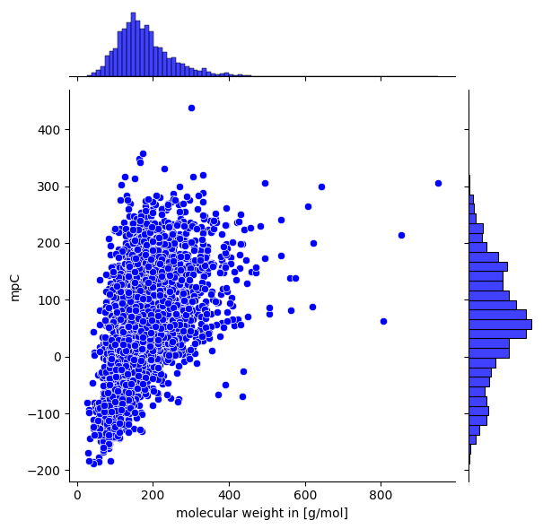
Molecular Weight against Target
Another option for visual analysis is to plot the molecule weight against the target attribute. This might give an indication on how molecule size correlates with the target, often a usual observation.
[12]:
from grape_chem.plots import mol_weight_vs_target
print(data.target)
mol_weight_vs_target(data.smiles, data.target, save_fig=True, fig_height=6, target_name='mpC')
[-161.51 94.8 239.75 ... 176. 65. -34. ]
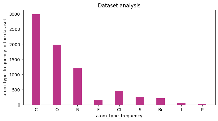
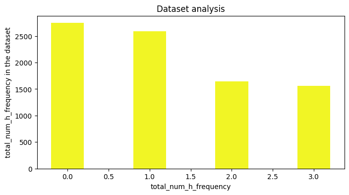
Feature number charts
If only a basic analysis of the dataset, is needed, then one can generate number charts based on the featurizion of the molecules. The implementation is built on top of DGL-LIFESCI analyze_mols function (github), below is an example.
[13]:
%matplotlib inline

results, figures = data.analysis(download=True, plots=['atom_type_frequency','total_num_h_frequency'], fig_size=[8,4],
                                 save_plots=True)
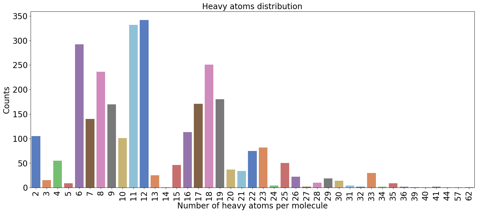
We could also plot the number of heavy atoms as a barchart:
[14]:
from grape_chem.plots import num_heavy_plot
num_heavy_plot(data.smiles, fig_size=(20,8))
[14]:
<Axes: title={'center': 'Heavy atoms distribution'}, xlabel='Number of heavy atoms per molecule', ylabel='Counts'>
Clustering and data splitting
There are several ways to split the graph dataset into the training, validation and testing splits, including random, stratified or by molecular weight. A more interesting addition in this toolbox is a split based on Butina clustering [2], where the molecules are clustered based on the Morgan Fingerprint and the Tanimoto similarity. Within there are two options: (1) a uniform split where we sample across all clusters evenly, and (2) a realistic split where we fill up the train., val. and test. split with clusters from largest to smallest in order.
Below, we choose the realistic split:
[15]:
from grape_chem.datasets import BradleyDoublePlus
data = BradleyDoublePlus()

train, val, test = data.split_and_scale(scale=True, split_type='butina_realistic', seed=42, is_dmpnn=True);
100%|██████████| 2402/2402 [00:00<00:00, 4044.18it/s]
100%|██████████| 292/292 [00:00<00:00, 3589.26it/s]
100%|██████████| 295/295 [00:00<00:00, 3060.39it/s]
Note that we scale using the training set immediately and that we specify that we are working with DMPNN (a directional GNN).
GNN Models
With the data loaded, filtered, featurized and split, let’s define a Graph Neural Network and test it! We can always find the number of features like thus:
[16]:
print(f'Node feature dimension: {data.num_node_features}')
print(f'Edge feature dimension: {data.num_edge_features}')
Node feature dimension: 44
Edge feature dimension: 12
Model definition
To define a model, all we need to do is load one of the in-built models like MPNN or MEGNet and apply it. Any model that can handle the PyG graphs as input would work for that matter, fx. one could use the PyG models instead. Below, we load the DMPNN model directly from the package and initialize it:
[17]:
from grape_chem.models import DMPNN
import torch

node_hidden_dim = 64
batch_size = 32
mlp_layers = [512, 256, 128]


model = DMPNN(node_in_dim=data.num_node_features, edge_in_dim=data.num_edge_features, node_hidden_dim=node_hidden_dim,
              mlp_out_hidden=mlp_layers)


print('Full model:\n--------------------------------------------------')
print(model)

device = torch.device('cpu')
Full model:
--------------------------------------------------
DMPNN(
  (rep_dropout): Dropout(p=0.0, inplace=False)
  (encoder): DMPNNEncoder(
    (act_func): ReLU()
    (W1): Linear(in_features=56, out_features=64, bias=True)
    (W2): Linear(in_features=64, out_features=64, bias=True)
    (W3): Linear(in_features=108, out_features=64, bias=True)
    (dropout_layer): Dropout(p=0.15, inplace=False)
  )
  (mlp_out): Sequential(
    (0): Linear(in_features=64, out_features=512, bias=True)
    (1): ReLU()
    (2): Linear(in_features=512, out_features=256, bias=True)
    (3): ReLU()
    (4): Linear(in_features=256, out_features=128, bias=True)
    (5): ReLU()
    (6): Linear(in_features=128, out_features=1, bias=True)
  )
)
Loss and Optimizer
Like with any deep learning model, we define a loss function and optimizer.
[18]:
from torch import nn

loss_func = nn.functional.mse_loss
optimizer = torch.optim.Adam(model.parameters(), lr=1e-3, weight_decay=1e-6)
We can additionally define an Early Stopper to help improve the output:
[19]:
from grape_chem.utils import EarlyStopping
early_stopper = EarlyStopping(patience=30, model_name='best_model')
As well as a scheduler to reduce the learning-rate whenever the training hits a plateau:
[20]:
from torch.optim import lr_scheduler
scheduler = lr_scheduler.ReduceLROnPlateau(optimizer, mode='min', factor=0.9, min_lr=0.0000000000001, patience=15)
Training
Here, we just use the previous determined training and validation splits to train the model inside the train_model function:
[21]:
from grape_chem.utils import train_model

train_loss, val_loss = train_model(model = model,
                                  loss_func = 'mse',
                                  optimizer = optimizer,
                                  train_data_loader= train,
                                  val_data_loader = val,
                                  batch_size=batch_size,
                                  epochs=300,
                                  early_stopper=early_stopper,
                                   scheduler=scheduler)

model.load_state_dict(torch.load('best_model.pt'))
epoch=46, training loss= 0.093, validation loss= 0.427: 15%|█▌ | 46/300 [00:14<01:20, 3.16it/s]
Early stopping reached with best validation loss 0.3590
Model saved at: best_model.pt
[21]:
<All keys matched successfully>
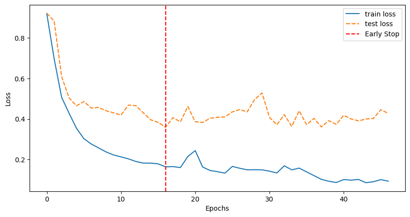
Loss plot
The training function returns the training and validation losses which can visualize as:
[22]:
from grape_chem.plots import loss_plot
loss_plot([train_loss, val_loss], ['train loss', 'test loss'], early_stopper.stop_epoch)
Testing and Post-processing
For testing, we use the test_model from the toolbox which essentially just uses predicts the test SMILES using the trained model:
[23]:
from grape_chem.utils import test_model
preds = test_model(model=model,
                   test_data_loader=test)
100%|██████████| 10/10 [00:00<00:00, 178.52it/s]
Then we calculate some (re-scaled) metrics on the predictions using pred_metric:
[24]:
from grape_chem.utils import pred_metric
pred_metric(prediction=preds,target=test.y, metrics='all', print_out=True, rescale_data=data);
MSE: 3788.606
RMSE: 61.552
SSE: 1117638.819
MAE: 49.257
R2: 0.629
MRE: 64.075%
MDAPE: 28.588%
Note that we have to pass the original data object to make sure we are recaling on the correct data.
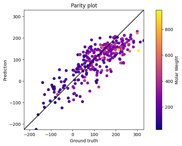
Parity and Residual plots
We could also choose to plot the parity and residual plots:
[25]:
from grape_chem.plots import parity_plot, residual_plot
# We rescale the predictions and ground truth before plotting
preds_rescaled, test_y_rescaled = data.rescale_data(preds), data.rescale_data(test.y)
parity_plot(prediction=preds_rescaled,target=test_y_rescaled, mol_weights=test.mol_weights);
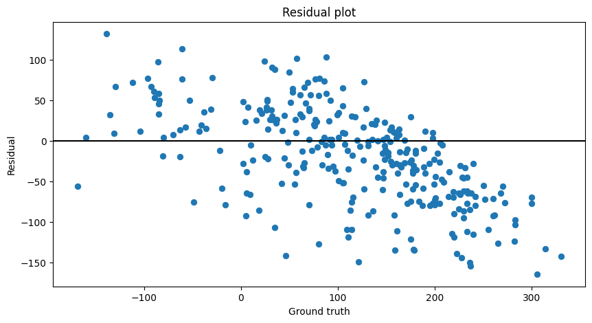
[26]:
residual_plot(prediction=preds_rescaled,target=test_y_rescaled)
[26]:
<Axes: title={'center': 'Residual plot'}, xlabel='Ground truth', ylabel='Residual'>
Metrics
We can also examine the how the over splits, training and validation, behave. To do so, we might calculate average or overall metrics:
[27]:
# Generating the predictions

train_preds = test_model(model=model,test_data_loader=train)
val_preds = test_model(model=model,test_data_loader=val)
test_preds = test_model(model=model,test_data_loader=test)
100%|██████████| 76/76 [00:00<00:00, 442.06it/s]
100%|██████████| 10/10 [00:00<00:00, 370.22it/s]
100%|██████████| 10/10 [00:00<00:00, 448.13it/s]
[28]:
# Overall R2

overall = 0
overall += pred_metric(prediction=train_preds,target=train.y, metrics='r2', print_out=False)['r2']
overall += pred_metric(prediction=val_preds,target=val.y, metrics='r2', print_out=False)['r2']
overall += pred_metric(prediction=test_preds,target=test.y, metrics='r2', print_out=False)['r2']
print(f'Overall R2: {overall/3}')
Overall R2: 0.7306092634540665
[29]:
# Overall MAE

overall = 0
overall += pred_metric(prediction=train_preds,target=train.y, metrics='mae', print_out=False, rescale_data=data)['mae']
overall += pred_metric(prediction=val_preds,target=val.y, metrics='mae', print_out=False, rescale_data=data)['mae']
overall += pred_metric(prediction=test_preds,target=test.y, metrics='mae', print_out=False, rescale_data=data)['mae']
print(f'Overall MAE: {overall/3}')
Overall MAE: 40.01786928641531
Residual Density
Furthermore, using the predictions from all three splits we can plot the residual density:
[30]:
from grape_chem.plots import residual_density_plot
residual_density_plot(train_pred=train_preds, val_pred=val_preds, test_pred=test_preds,
                      train_target=train.y, val_target=val.y, test_target=test.y)
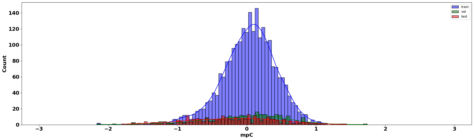
For the (scaled) residual density plot, we are looking to examine how our errors or residuals behave. Namely, we want them to be normally distributed, and they seem to be!
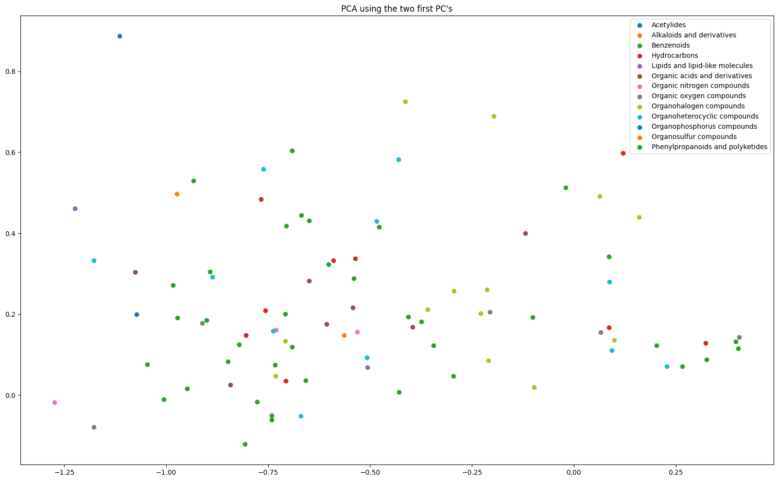
Latent analysis
PCA
Finally, we could analyze the model latents by applying a PCA model and plotting them based on groups. Let us first classify a subset of our test SMILES and label them according to their classes:
[31]:
from grape_chem.analysis import classyfire, classyfire_result_analysis
ids, data_ids = classyfire(test.smiles[:100], log=False)
# -> ids are used for the result analysis and data_ids for specifying the data point from the test set we can use

class_dict, smile_dict, rel_ids = classyfire_result_analysis(idx=ids, layer=1, return_relative_ids=True)
Found log file in working directory.
All passed smiles are already in the passed log_file.
Key error occurred using superclass for file 683.json.
Key error occurred using superclass for file 695.json.
Key error occurred using superclass for file 656.json.
Key error occurred using superclass for file 640.json.
Key error occurred using superclass for file 660.json.
Key error occurred using superclass for file 621.json.
Key error occurred using superclass for file 699.json.
Key error occurred using superclass for file 676.json.
[32]:
indices = list(class_dict.keys())
labels = list(class_dict.values())
print(labels[:10])
['Benzenoids', 'Benzenoids', 'Benzenoids', 'Benzenoids', 'Phenylpropanoids and polyketides', 'Benzenoids', 'Organic nitrogen compounds', 'Organophosphorus compounds', 'Organoheterocyclic compounds', 'Organoheterocyclic compounds']
This will let us label the PCA plot much better. Now we can retrieve and generate the PCA plot:
[33]:
lats_data = test[:100]
preds, lats = test_model(model, test_data_loader=lats_data, return_latents=True)
lats = lats.cpu().detach().numpy()
100%|██████████| 4/4 [00:00<00:00, 317.61it/s]
[34]:
from grape_chem.plots import pca_2d_plot
pca_2d_plot(latents=lats[rel_ids], labels=labels, save_fig=True, fig_size=(20,12))
[34]:
<Axes: title={'center': "PCA using the two first PC's"}>
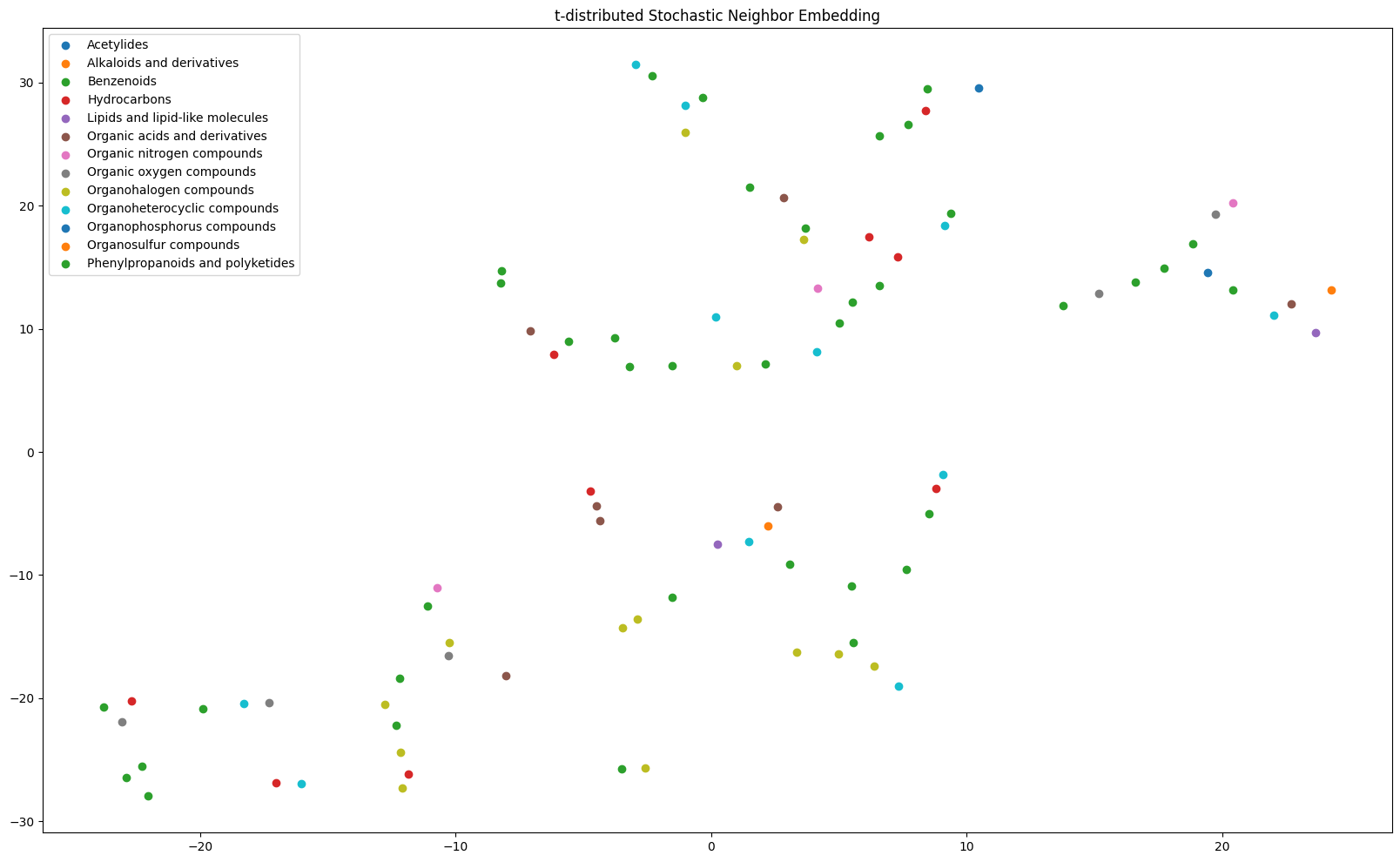
t-SNE
Alternatively, we could use the t-SNE (t-distributed Stochastic Neighbor Embedding) algorithm by [4] to perform dimensionality reduction. The algorithm essentially uses probabilistic similarity measures to cluster the input point for n-components (here 2) and relies on two hyperparameters: perplexity (approximately equal to the number of neighbors per point) and the number of iterations the algorithm runs for.
It is generally a tricky feat to have the algorithm converge and produce interesting results, but it is possible! Here is an example use:
[35]:
from grape_chem.plots import tSNE_plot
tSNE_plot(latents=lats[rel_ids], labels=labels, perplexity=5, save_fig=True, fig_size=(20,12))
[35]:
<Axes: title={'center': 't-distributed Stochastic Neighbor Embedding'}>
Prediction
The final step of the typical machine learning pipeline is to use the model for prediction. This is made easy by the DataSet method predict_smiles. The requirement for the method to work is that (1) the model and dataset share the same node- and edge-features (generally true if the model was trained using a specific DataSet object’s data); and (2) that the input SMILES are valid compounds and recognized by rdkit.
Using it looks like the following:
[36]:
SMILES_to_predict = ['CC','CCO', 'CCCCCC']
data.predict_smiles(SMILES_to_predict, model) # The results are in degrees Celsius
[36]:
{'CC': -244.16973876953125,
 'CCO': -88.8644027709961,
 'CCCCCC': -118.04553985595703}
Note that the results can only be rescaled if DataSet has internal mean and std value, or they have to be passed manually.
For completion, here is what it looks like to predict from a dataset without first training the model (using the FreeSolv dataset and AFP as an example):
[37]:
from grape_chem.datasets import FreeSolv
from grape_chem.models import AFP

data = FreeSolv()
model = AFP(node_in_dim=data.num_node_features, edge_in_dim=data.num_edge_features)
data.predict_smiles(['CC', 'CCCCCCCCC'], model)
[37]:
{'CC': 0.0484485849738121, 'CCCCCCCCC': 0.05039355903863907}
These numbers are just random, of course.
References
[1] Jean-Claude Bradley and Andrew Lang and Antony Williams, Jean-Claude Bradley Double Plus Good (Highly Curated and Validated) Melting Point Dataset, 2014, http://dx.doi.org/10.6084/m9.figshare.1031637
[2] Feunang, Y., Eisner, R., Knox, C., Chepelev, L., Hastings, J., Owen, G., Fahy, E., Steinbeck, C., Subramanian, S., Bolton, E., Greiner, R., & Wishart, D. S. (2016). ClassyFire: automated chemical classification with a comprehensive, computable taxonomy. Journal of Cheminformatics, 8(1), 61. https://doi.org/10.1186/s13321-016-0174-y
[3] Butina, D. (1999). Unsupervised Data Base Clustering Based on Daylight’s Fingerprint and Tanimoto Similarity: A Fast and Automated Way To Cluster Small and Large Data Sets. Journal of Chemical Information and Computer Sciences, 39(4), 747-750. https://doi.org/10.1021/ci9803381
[4] van der Maaten, L., & Hinton, G. (2008). Visualizing data using t-sne. Journal of Machine Learning Research, 9 (86), 2579–2605. http://jmlr.org/papers/v9/vandermaaten08a.html
Extra Code to generate PDFs:
[2]:
#PDF conversion code
!export PATH=/Library/TeX/texbin:$PATH
!jupyter nbconvert 'GraPE-Chem Demonstration'.ipynb --to pdf --no-prompt
[NbConvertApp] Converting notebook GraPE-Chem Demonstration.ipynb to pdf
[NbConvertApp] Support files will be in GraPE-Chem Demonstration_files/
[NbConvertApp] Making directory ./GraPE-Chem Demonstration_files
[NbConvertApp] Writing 80126 bytes to notebook.tex
[NbConvertApp] Building PDF
[NbConvertApp] Running xelatex 3 times: ['xelatex', 'notebook.tex', '-quiet']
[NbConvertApp] Running bibtex 1 time: ['bibtex', 'notebook']
[NbConvertApp] WARNING | bibtex had problems, most likely because there were no citations
[NbConvertApp] PDF successfully created
[NbConvertApp] Writing 663584 bytes to GraPE-Chem Demonstration.pdf
[ ]: